Building an End-to-End FPL Data Pipeline

Background

Football has always been one of my biggest interests, and I have been an Arsenal (Champions of England) supporter for as long as I can remember. Naturally, that interest eventually led me to Fantasy Premier League (FPL).

For anyone unfamiliar with it, FPL is a fantasy football game based on the English Premier League. You create a virtual squad of real-life players and earn points based on what they do in actual matches. Goals, assists, clean sheets, and saves can earn you points, while things like cards, missed penalties, and conceding goals can quickly ruin your weekend.

A group of friends and I run a competitive private league, with money on the line at the start of each season. As the competition grew, I wanted to make more informed decisions about player selections, transfers, fixtures, and form instead of relying entirely on gut feeling (which, as it turns out, is not always a great strategy).

I initially built a dashboard for my own analysis. After sharing it with my friends and seeing them use it, I decided to take it further. The dashboard eventually evolved into an automated data pipeline that refreshes with new FPL data each gameweek, turning a personal fantasy football tool into a complete data engineering project.

What I Built

The end result is an end-to-end ETL pipeline that starts with the FPL API and ends with structured data ready for analysis and visualization.

The workflow is split into three main stages:

1. Extract raw data from the FPL API.
2. Transform it into cleaner tables and useful metrics.
3. Load everything into PostgreSQL.

Apache Airflow handles the orchestration, while Python handles most of the data processing. Docker packages the services together, and Power BI sits at the end of the pipeline as the reporting layer.

Here is a simplified example of how the pipeline starts by pulling data from the FPL API:

import requests
import pandas as pd

API_BASE_URL = "https://fantasy.premierleague.com/api/"

response = requests.get(f"{API_BASE_URL}bootstrap-static/")
data = response.json()

players = pd.DataFrame(data["elements"])
teams = pd.DataFrame(data["teams"])
events = pd.DataFrame(data["events"])

Once the data is collected, the pipeline cleans it, standardizes column names, and prepares the output tables for PostgreSQL. The goal is to take raw API responses and turn them into something that is actually pleasant to query and visualize.

The Data Source

The main data source for this project is the official Fantasy Premier League API. It provides pretty much everything needed for analysis: players, teams, fixtures, gameweeks, and a whole lot of statistics that can be used to justify why my latest transfer was definitely not a terrible decision.

The pipeline focuses on a few key areas:

• Player attributes and current form
• Team strengths and fixture difficulty
• Gameweek-level information
• Match stats such as goals, assists, cards, and saves

For the initial extraction, I use the bootstrap-static endpoint. It contains the latest static information needed for the main analysis, making it a good starting point for the pipeline.

response = requests.get(f"{API_BASE_URL}bootstrap-static/")
bootstrap_data = response.json()

players_df = pd.DataFrame(bootstrap_data["elements"])
teams_df = pd.DataFrame(bootstrap_data["teams"])
fixtures_df = pd.DataFrame(bootstrap_data["fixtures"])

Once the data is extracted, the pipeline removes irrelevant columns, renames fields for clarity, and creates additional tables for reporting. This is particularly important for player and fixture data, where the raw API structures are not always immediately ready for analysis.

Architecture Overview

The overall architecture is pretty straightforward: data comes in from the FPL API, gets processed and organized, and eventually ends up in PostgreSQL for analysis and reporting.

What the Raw Data Looks Like

One of the more interesting parts of this project was seeing what the raw API data actually looked like before the pipeline started cleaning everything up.

At first glance, the data is already fairly usable. A simplified player record might look something like this:

{
  "id": 1,
  "web_name": "Salah",
  "team": 14,
  "total_points": 180,
  "now_cost": 13,
  "form": "4.8",
  "minutes": 2200
}

Pretty good, right? But once you start working with the full API response, things get a little messier. Different fields use different formats, some values need to be converted, and IDs like team: 14 are not particularly useful when you’re trying to understand which actual team the player belongs to.

The pipeline cleans and organizes this information into structured columns containing player identifiers, form, cost, team associations, and performance metrics. These cleaned tables then become the foundation for the dashboards and deeper analysis later on.

Data Modeling

The database design was shaped by one pretty simple idea: keep the data structured enough for reporting, but flexible enough to support future analysis. Instead of putting everything into one massive table (which would have been a nightmare to work with), I split the data into domain-specific tables.

A simplified version of the schema looks like this:

CREATE TABLE players (
  player_id INT PRIMARY KEY,
  web_name VARCHAR(100),
  team INT,
  total_points INT,
  now_cost INT,
  form FLOAT
);

CREATE TABLE fixtures (
  fixture_id INT PRIMARY KEY,
  GW_id INT,
  home_team_id INT,
  away_team_id INT,
  home_team_score INT,
  away_team_score INT
);

CREATE TABLE events (
  GW_id INT PRIMARY KEY,
  name VARCHAR(100),
  finished BOOLEAN,
  average_GW_score FLOAT
);

This structure makes it easier to answer questions like: Which players performed well this week? Or: How did team strengths affect fixture outcomes?

Code - Transforming the Data

The raw API response had nested structures, inconsistent naming, and plenty of columns that I didn’t actually need. So I used Python and pandas to clean everything up before loading it into the database.

import pandas as pd

players_df = pd.DataFrame(bootstrap_data["elements"])
players_df = players_df.rename(columns={"id": "player_id", "web_name": "web_name"})
players_df = players_df[["player_id", "web_name", "team", "total_points", "now_cost", "form"]]

The basic idea was pretty simple: take a huge amount of raw data and keep only what was actually useful. Fixtures were a little more complicated. The raw data included nested match statistics, so I transformed those into cleaner summary tables covering things like goals, assists, cards, and saves.

This step was important because Power BI works much better when the data is already organized into clean rows and columns. Basically, I wanted to do the messy work in Python first instead of making Power BI deal with an inconsistent data structure.

Loading the Data to the PostgreSQL Database

Once the data was cleaned, it was time to get it into PostgreSQL. Each CSV was loaded into its own relational table, with each table serving a specific purpose in the overall project.

The main tables are:

• players: player-level attributes and current performance
• fixtures: match and gameweek context
• events: gameweek summaries
• fixtures_stats_overview: aggregated fixture statistics
• fixtures_stats_eachplayer: player-specific match events
• teams: team metadata and strength ratings
• positions: player position categories
• minileague: league and entry performance details

A simplified load example looks like this:

import psycopg2

conn = psycopg2.connect(DATABASE_URL)
cur = conn.cursor()

for row in players_df.itertuples():
    cur.execute(
        """
        INSERT INTO players (player_id, web_name, team, total_points, now_cost, form)
        VALUES (%s, %s, %s, %s, %s, %s)
        """,
        (row.player_id, row.web_name, row.team, row.total_points, row.now_cost, row.form),
    )

conn.commit()

Once the data was loaded, PostgreSQL became the central source of truth for everything downstream. Instead of having the dashboard depend on a bunch of separate CSV files, all the cleaned data could be queried from one structured database.

Much cleaner. Much easier to maintain. And significantly less likely to make me question my life choices when I needed to update something.

Orchestration with Airflow

Fantasy Premier League is constantly changing. Player values shift, fixtures get updated, and new gameweek results arrive every week. That means a dashboard can become outdated pretty quickly if the data is not refreshed regularly.

This is where Airflow come in. I wanted to stop manually running each step of the pipeline every time new data became available. Airflow allowed me to define the workflow, connect the different tasks, and run everything in the right order.

The DAG structure looks like this:

from airflow import DAG
from airflow.operators.python import PythonOperator

with DAG("fpl_api_flow", schedule_interval=None, catchup=False) as dag:
    task1 = PythonOperator(task_id="initialize_db", python_callable=run_initialize_db)
    task2 = PythonOperator(task_id="extract_transform_load", python_callable=run_extract_transform_load)
    task3 = PythonOperator(task_id="load_csv_to_db", python_callable=run_load_csv_to_db)

    task1 >> task2 >> task3

The main goal was pretty simple: make the pipeline repeatable, observable, and easy to rerun whenever the data changed. Once scheduled, the pipeline can run regularly and keep the database closer to the latest FPL data.

Packaging and Querying the Data

Once the pipeline was working, I wanted the project to be reasonably easy to run without having to manually install and configure every individual service.

That is where Docker comes in.

The project packages the main components into containers:

• PostgreSQL for the warehouse
• Airflow webserver and scheduler for orchestration
• Python-based ETL code for processing the data

So you: clone the repository, configure the environment, and start the project without having to spend an entire afternoon wondering why one particular dependency refuses to install.

SQL then became the bridge between the database and the reporting layer. I used it to create tables, join data across different domains, and prepare information for analysis.

A simple example looks like this:

SELECT
  p.web_name,
  p.total_points,
  f.GW_id,
  f.home_team_id,
  f.away_team_id
FROM players p
JOIN fixtures f ON p.team = f.home_team_id
ORDER BY p.total_points DESC;

Queries like this helped me validate that the transformed tables were connected correctly and that the database could support the analysis required by the dashboard.

Power BI Dashboard

The dashboard is the final layer of the project. All the data that has been extracted, transformed, and loaded into PostgreSQL eventually ends up here.

The goal was to turn all of that data into something I could actually use when trying to make FPL decisions. Because having a database full of thousands of rows is great, but it is not particularly helpful when you are trying to decide whether transferring in a player is a big brain move or the beginning of another terrible gameweek.

Gameweek Stats

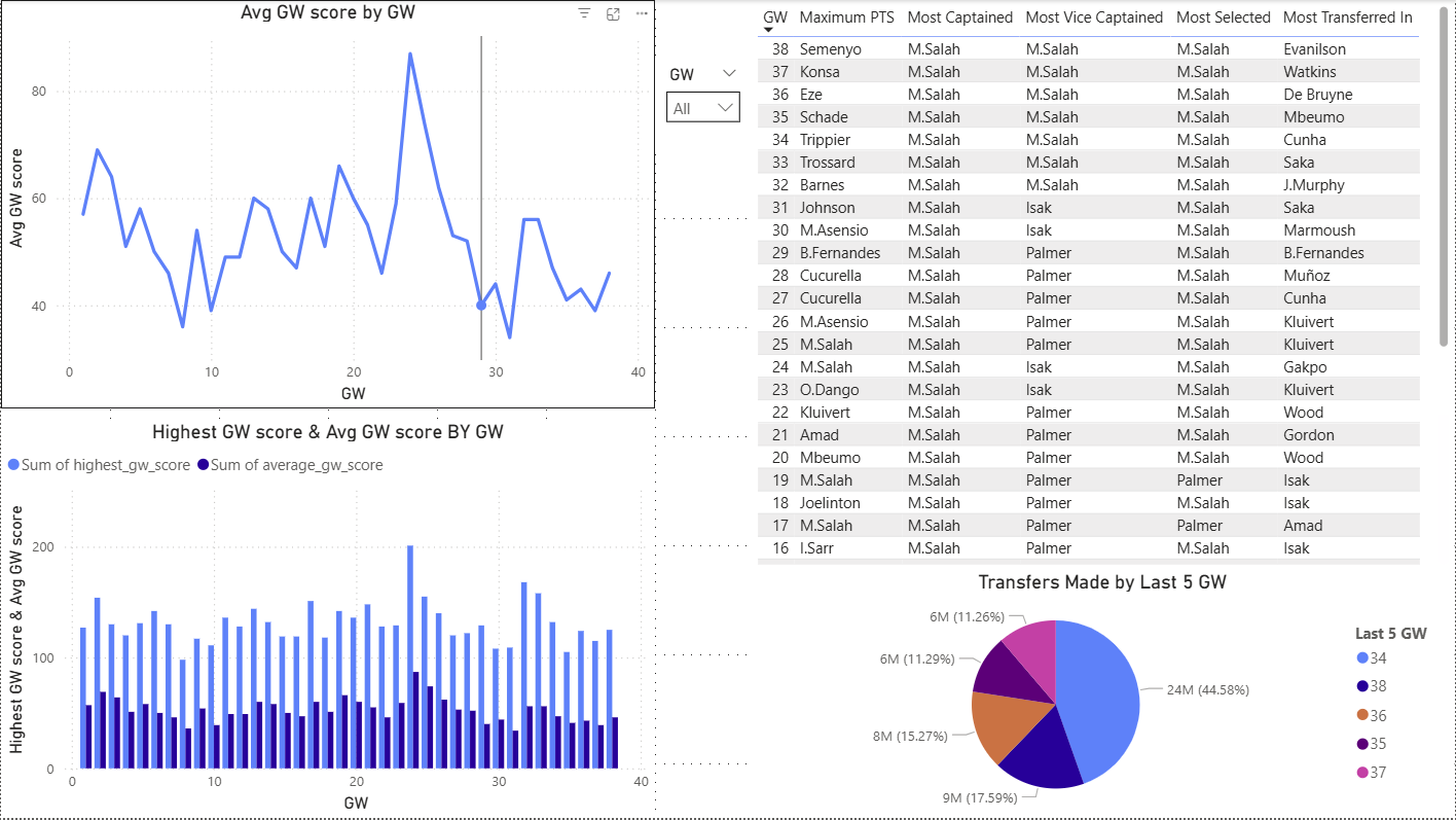
This page tracks performance across the season, showing average gameweek scores, the highest-scoring rounds, and how performance changed over time. It also shows the top performers and major events from each gameweek, including the highest points scored, most-captained players, and most-transferred-in players. This makes it easier to see which gameweeks were particularly strong, which players attracted the most attention, and how the season evolved over time.

Chips & Positions

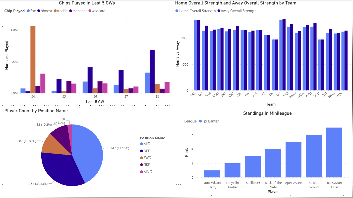
This view focuses on chip usage, team strength, and my private league standings. It tracks how managers used chips such as Wildcard, Triple Captain, and Bench Boost, while also comparing home and away team strength. The mini-league standings add the most important part of the analysis: seeing exactly how badly my friends were beating me.

Fixtures

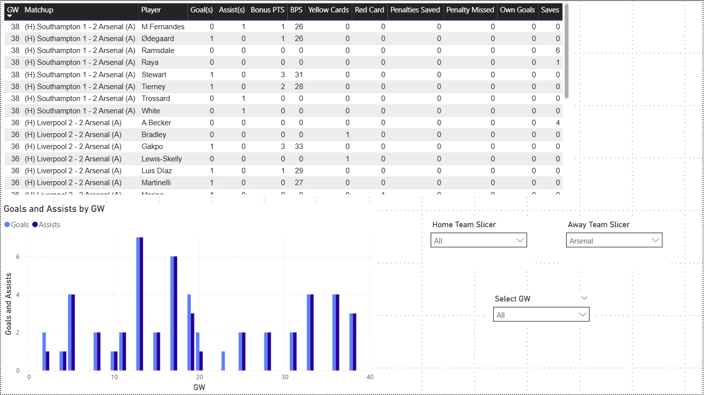
This section focuses on fixture-level analysis. Users can filter by home team, away team, and gameweek to explore individual matchups and results. The page also brings together goals, assists, and other fixture statistics, making it easier to compare team performance and understand the context behind upcoming and completed fixtures.

Player Stats

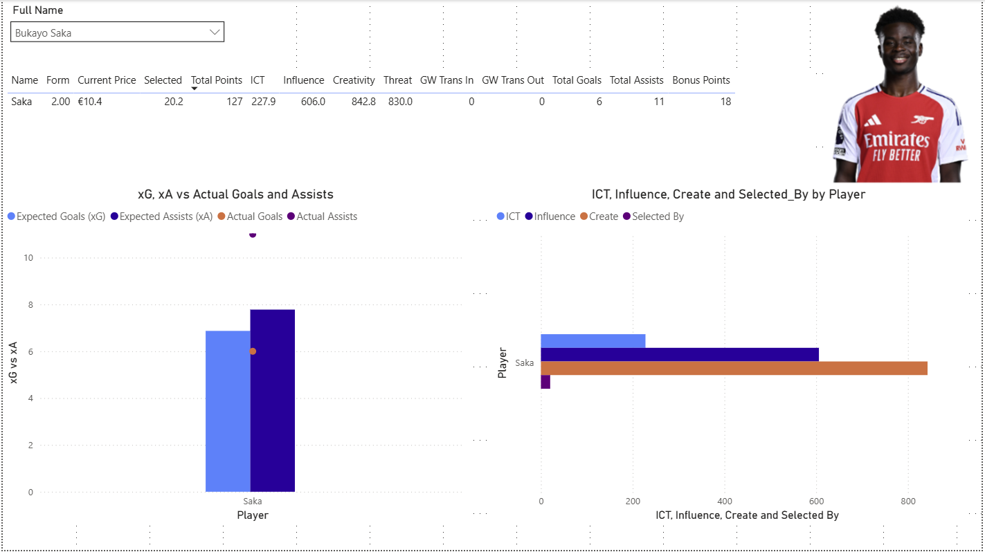
This page focuses on individual player performance. It compares actual goals and assists with expected goals (xG) and expected assists (xA), while also showing metrics such as ICT Influence, creativity, and how many managers selected a player. The goal was to make it easier to compare players from different angles. Sometimes the player with the most points is the obvious choice. Sometimes the underlying numbers suggest something different. And sometimes I ignore both and make a transfer based on vibes, which is usually when things go wrong.

What Went Wrong and What I Learned

This project was a pretty good learning experience, but it definitely had its share of pain points.

The biggest issue was that I initially treated the raw API structure too literally. It worked, but it made the transformation logic more brittle than it needed to be. Basically, I was building too much around the way the API happened to return the data instead of designing the structure around how I actually wanted to use it.

If I were building the project again, I would:

• Design the database schema earlier with reporting needs in mind
• Flatten nested data more aggressively before loading it
• Add stronger validation for missing or malformed API fields
• Focus each dashboard around a few high-value questions instead of trying to show everything at once

The biggest lesson for me was that data engineering is not just about collecting data and moving it from one place to another. The real value comes from building a workflow that is automated, structured, reliable, and connected to a clear goal.

In this case, that goal was pretty simple: turn FPL data into something that could actually help me make better decisions.

Whether it actually made me better at FPL is still up for debate.