Building a Speech Emotion Recognition System

Background

Voice carries a lot more information than just the words we say. Even when someone says the exact same sentence, you can usually tell whether they’re happy, angry, nervous, or sad just by the way they say it. That got me wondering: could a machine do the same thing? And yes… I definitely spent a little too much time recording random audio clips just to see if I could confuse the model.

What started as a machine learning experiment pretty quickly turned into a full application. After training a model to recognize emotions from speech, I built a Flask web app so anyone could upload or record audio and see the prediction directly from their browser.

Goal

The goal was pretty simple: build an end-to-end machine learning workflow that starts with raw audio recordings and ends with a web application that can predict emotions in just a few seconds.

Along the way, the project covers everything from preprocessing audio and extracting meaningful features to training the model and serving predictions through Flask.

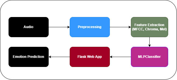
From a raw audio clip to a predicted emotion, this pipeline ties together the entire machine learning workflow.

Dataset

To train the model, I used the RAVDESS (Ryerson Audio-Visual Database of Emotional Speech and Song) dataset. Unlike image datasets where labels are usually stored in a separate CSV, RAVDESS keeps everything organized through its filename structure. That made parsing the labels surprisingly straightforward and meant I could build the training dataset directly from the audio files.

A filename like 03-01-02-01-01-01-01.wav tells you everything from the emotion being expressed to the actor who recorded it.

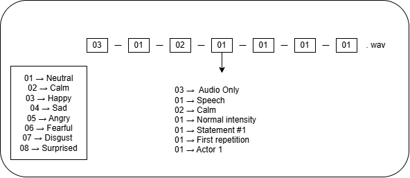
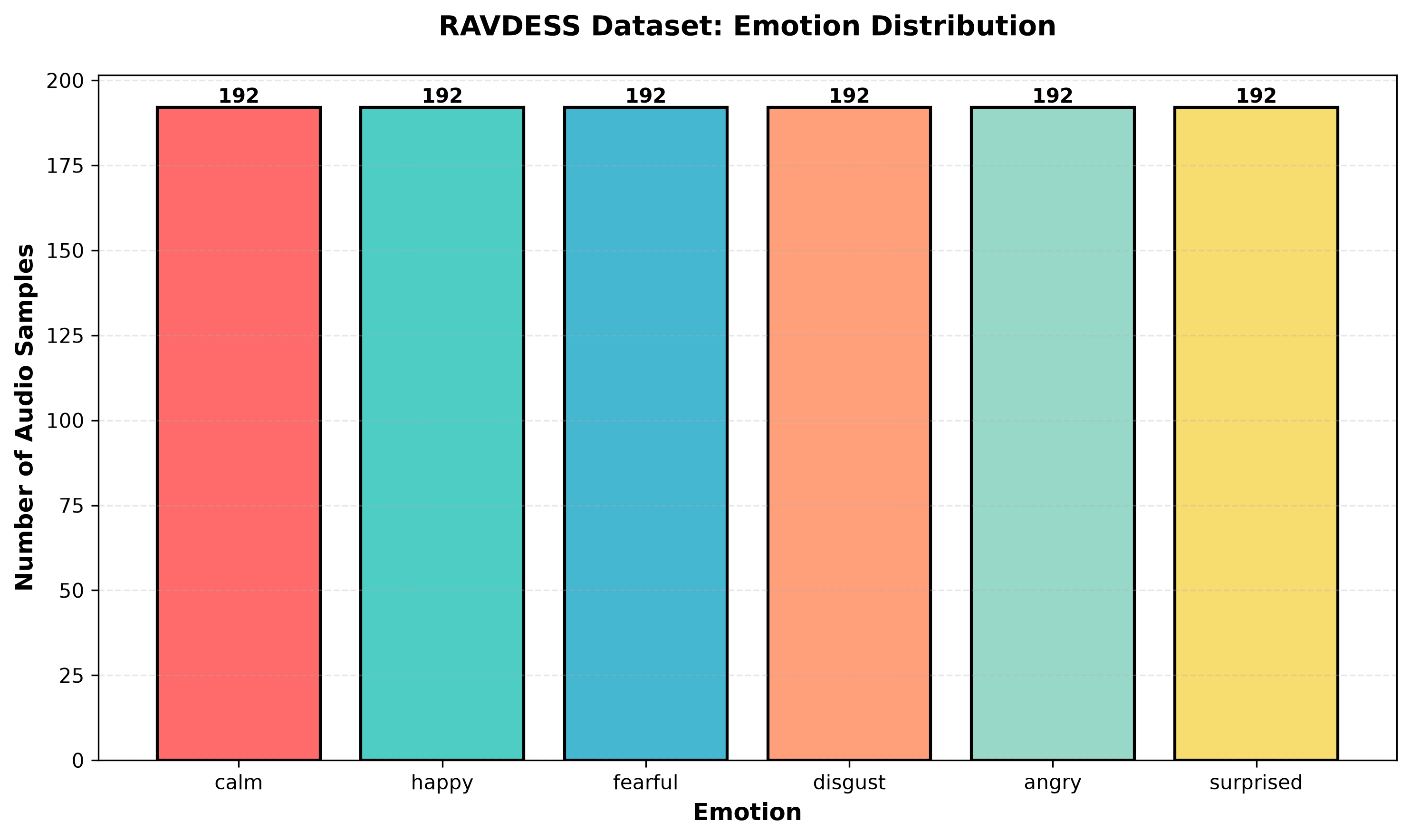
The original dataset contains recordings for all eight emotions, but for this project I focused on six of them. Each emotion has the same number of audio samples, giving the model a balanced dataset without one class dominating the others.

Having a balanced dataset is actually pretty important here. If one emotion appeared much more often than the others, the model could end up taking the easy way out by predicting that emotion more frequently. Since each class contains the same number of recordings, the model has to learn the actual differences in speech patterns instead.

Audio Preprocessing

Before the model could learn anything, the raw audio needed a bit of cleanup. Unlike images or tabular data, audio is just a stream of thousands of amplitude values, so the first step was making every recording consistent.

I loaded each WAV file, converted stereo recordings to mono when needed, and prepared the audio for feature extraction. This gave every sample a consistent starting point before extracting the information the model would actually learn from.

import soundfile as sf
import librosa

audio, sample_rate = sf.read(file_path, dtype='float32')
if audio.ndim > 1:
    audio = audio.mean(axis=1)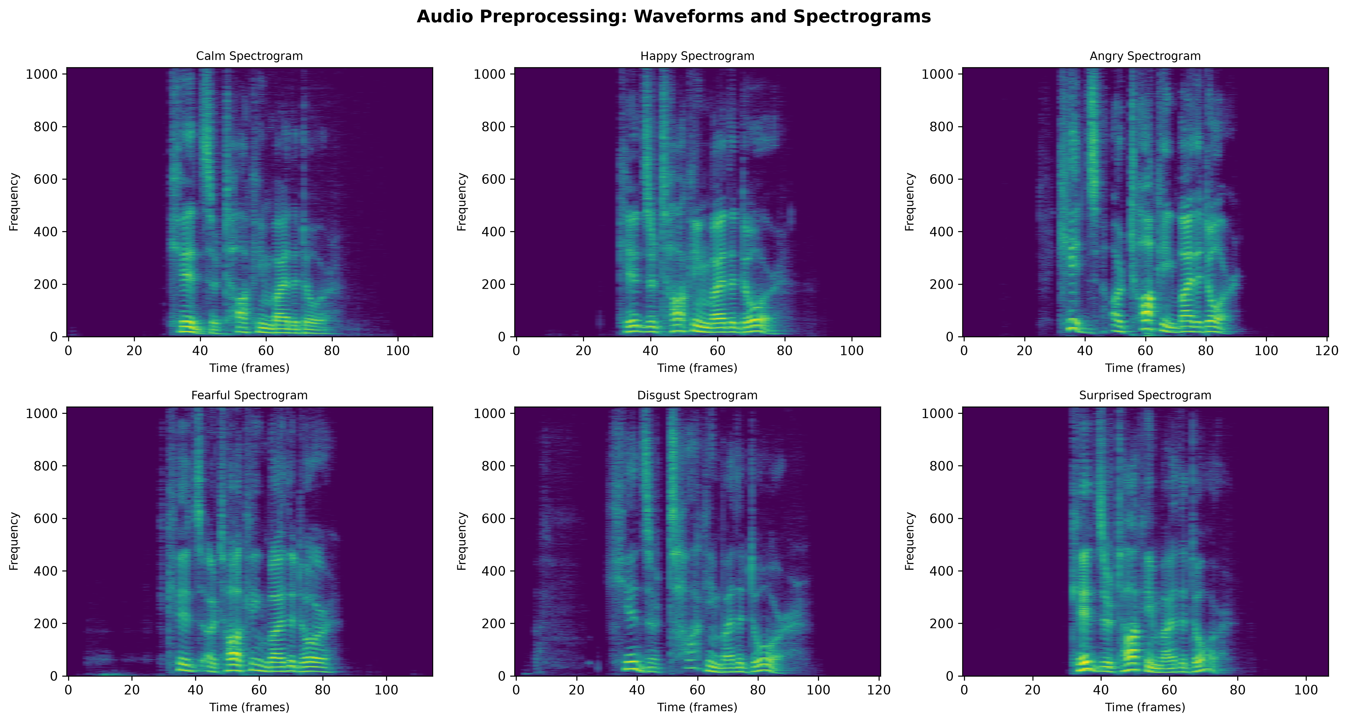

Even though two recordings may contain the same sentence, their waveforms and spectrograms can look surprisingly different depending on the emotion being expressed. These visualizations give a first glimpse into the patterns the model eventually learns to recognize.

A waveform shows how the audio signal changes over time, while a spectrogram reveals how energy is distributed across different frequencies. Since emotions affect things like pitch, loudness, and speaking rate, these visual differences become useful clues for the model.

Feature Extraction

Raw audio isn’t something a machine learning model can easily learn from. Instead of feeding thousands of waveform samples directly into the model, I extracted a set of features that capture the characteristics of a person’s voice while dramatically reducing the amount of data.

I used three common audio features:

• MFCCs to capture the overall shape and timbre of speech.
• Chroma features to represent the distribution of sound across different pitches.
• Mel spectrograms to summarize how energy changes across frequencies over time.

These features were combined into a single feature vector, which became the input for the classifier.

import numpy as np
import librosa

mfccs = np.mean(librosa.feature.mfcc(y=audio, sr=sr, n_mfcc=40).T, axis=0)
stft = np.abs(librosa.stft(audio))
chroma = np.mean(librosa.feature.chroma_stft(S=stft, sr=sr).T, axis=0)
mel = np.mean(librosa.feature.melspectrogram(y=audio, sr=sr).T, axis=0)
features = np.hstack((mfccs, chroma, mel))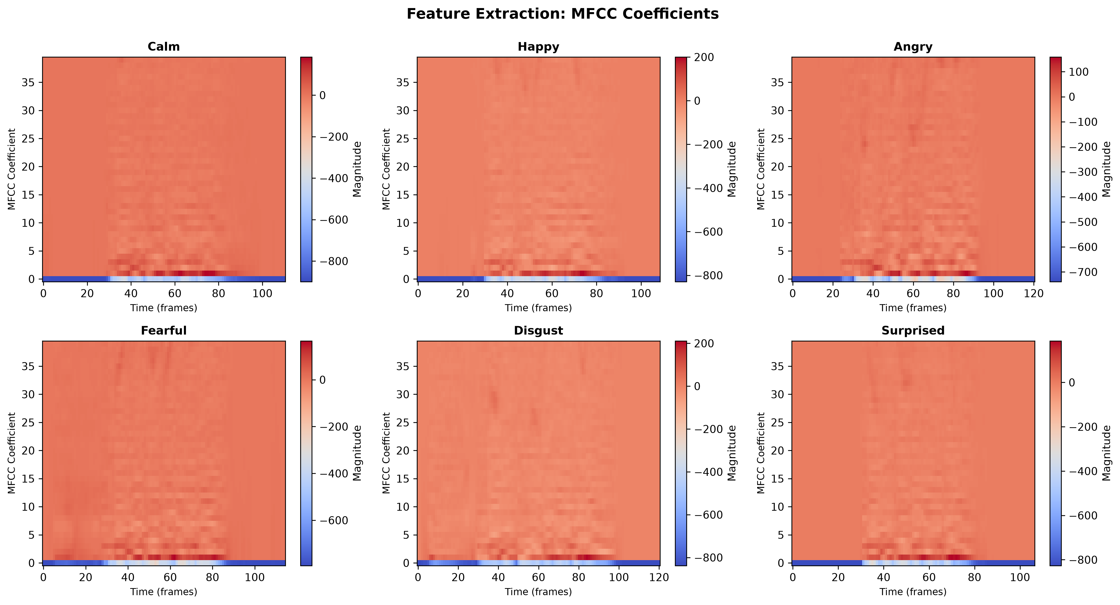

MFCCs transform raw audio into a compact numerical representation that preserves many of the characteristics of human speech. You can already see that different emotions produce noticeably different patterns, which gives the classifier something meaningful to learn from.

Training the Model

With the features extracted, the next step was training the classifier. I used an MLPClassifier (Multi-Layer Perceptron), which is a feed-forward neural network that’s well suited for structured feature vectors like MFCCs and mel spectrograms.

The dataset was split into 75% for training and 25% for testing, allowing me to evaluate how well the model performed on audio it hadn’t seen before.

from sklearn.neural_network import MLPClassifier
from sklearn.model_selection import train_test_split
from sklearn.metrics import accuracy_score

x_train, x_test, y_train, y_test = train_test_split(
  X, y, test_size=0.25, random_state=9
)

model = MLPClassifier(hidden_layer_sizes=(300,), max_iter=500)
model.fit(x_train, y_train)

y_pred = model.predict(x_test)
print(accuracy_score(y_test, y_pred))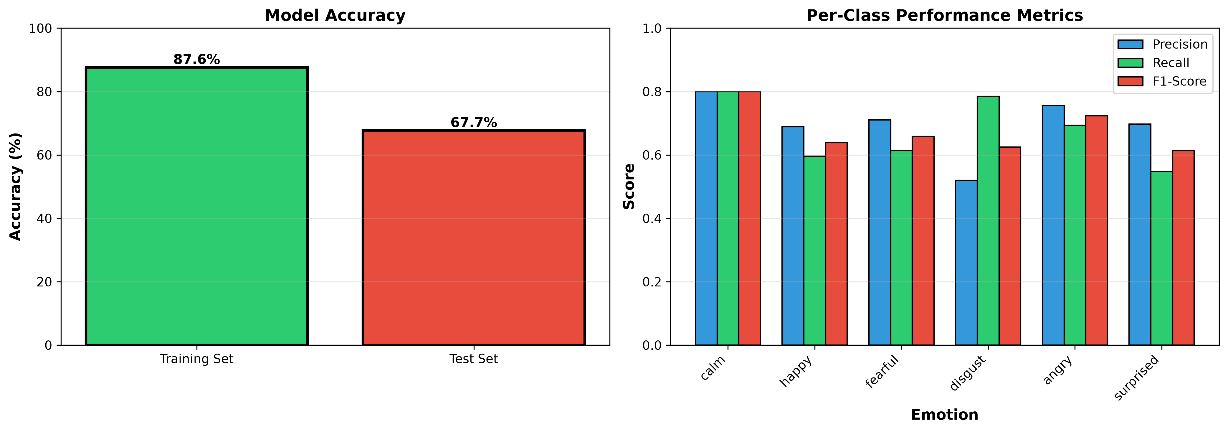

The model achieved 87.6% accuracy on the training set and 67.7% on the test set. While there's a noticeable gap between the two, that's fairly common with smaller datasets like RAVDESS and suggests the model learned some patterns that didn't fully generalize. It was a good reminder that evaluating on unseen data is much more important than looking at training accuracy alone.

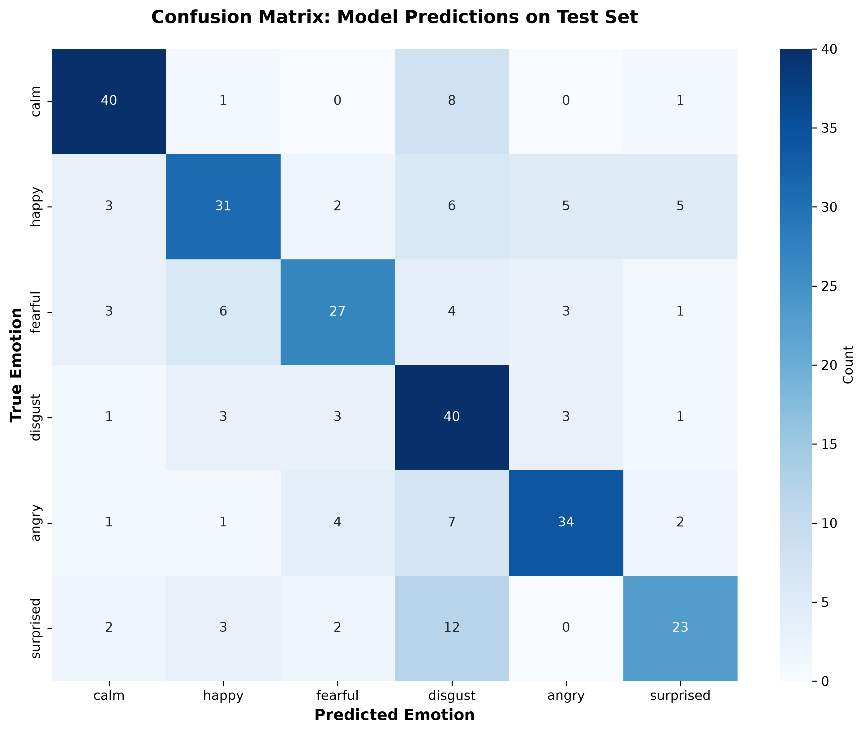
Looking beyond overall accuracy, the confusion matrix shows where the model struggled. Most emotions were classified correctly, but pairs like fearful vs. surprised were confused more often since they can share similar vocal characteristics. Interestingly, calm and disgust were among the easiest emotions for the model to recognize.

One thing I found pretty interesting was that the model’s mistakes often made sense from a human perspective too. Some emotions naturally sound similar, so it’s not surprising that the classifier occasionally mixed them up.

Bringing the Model to Life

Training the model was only half the project. A model sitting in a Jupyter notebook isn’t very useful, so I wanted to turn it into something people could actually interact with.

I built a Flask web application that lets users upload or record a short audio clip directly from their browser. Behind the scenes, the app runs the exact same preprocessing and feature extraction pipeline before passing the audio to the trained model and displaying the predicted emotion.

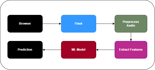
Once deployed, the model becomes just one part of the application. Every uploaded audio clip goes through the same preprocessing and feature extraction pipeline before the prediction is returned to the user.

from flask import Flask, render_template, request
from predict import emotion_prediction

app = Flask(__name__)

@app.route('/')
def index():
    return render_template('index.html')

@app.route('/predict', methods=['POST'])
def predict_func():
    file = request.files['filename']
    emotion, confidence, test_accuracy = emotion_prediction(file)
    return render_template('predict.html', emotion=emotion, confidence=confidence, test_accuracy=test_accuracy)

Final Experience

The final result is a lightweight web application that brings the entire pipeline together. Instead of stopping with a trained model, I wanted to build something that people could actually interact with. Users can record or upload an audio clip, submit it to the model, and get an emotion prediction in just a few seconds.

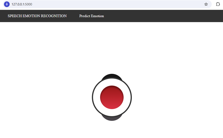
The landing page keeps things simple. Users can either record audio directly in the browser or upload an existing recording before sending it to the model for prediction.

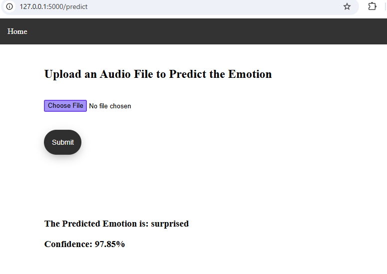
After processing the audio, the app displays the predicted emotion along with the model's confidence score.

What I Learned

This project taught me that building a machine learning model is only one part of the process. Just as important is everything around it - preparing the data, extracting meaningful features, evaluating the results, and packaging the model into something people can actually use.

It also gave me a much better understanding of how speech can be represented numerically. Concepts like MFCCs and mel spectrograms felt abstract at first, but seeing them improve emotion classification made it much clearer why they’re widely used in speech processing.